1. 实验2 图像的基本处理
1.1. 学习目标
- 了解图像的加法、混合操作
- 掌握图像的缩放,平移,旋转等
- 了解数字图像的仿射变换和透射变换
1.2. 实验内容
1.2.1. 算数操作
使用
OpenCV的cv.add()函数把两幅图像相加,或者可以简单地通过numpy操作添加两个图像,如 res = img1 + img2。两个图像应该具有相同的大小和类型,或者第二个图像可以是标量值。- 注意:
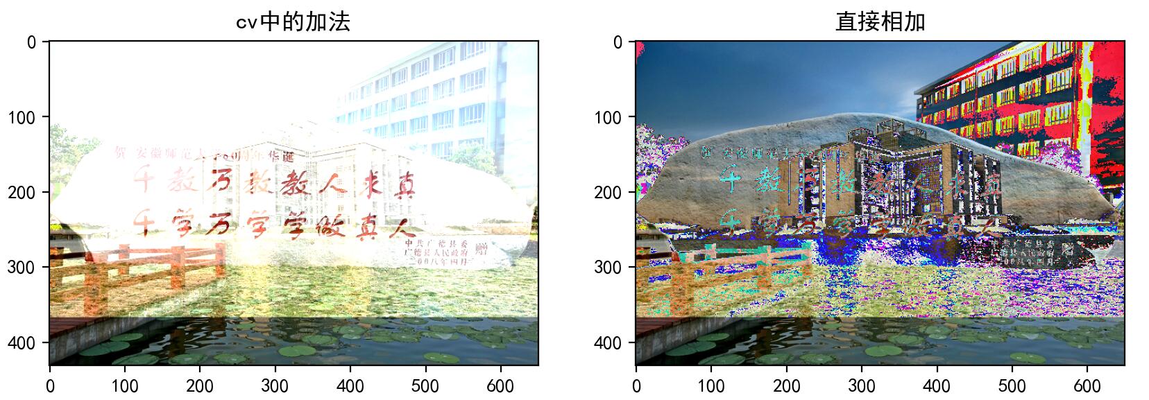
OpenCV加法和Numpy加法之间存在差异。 OpenCV的加法是饱和操作,而Numpy添加是模运算
>>> import numpy as np
>>> import cv2 as cv
>>> x = np.uint8([250])
>>> y = np.uint8([10])
>>> print( cv.add(x,y) ) # 250+10 = 260 => 255
[[255]]
>>> print( x+y )         # 250+10 = 260 % 256 = 4
[4]
这种差别在你对两幅图像进行加法时会更加明显。
OpenCV的结果会更好一点。所以我们尽量使用OpenCV中的函数。import numpy as np import cv2 as cv from matplotlib import pyplot as plt import matplotlib matplotlib.rcParams["font.sans-serif"]=["SimHei"] img1 = cv.imread("./images/001.jpg") img2 = cv.imread("./images/003.jpg") img2.resize(img1.shape) img3 =cv.add(img1,img2) img4 = img1 + img2 fig,axes = plt.subplots(nrows=1,ncols=2,figsize=(10,8),dpi=100) axes[0].imshow(img3[:,:,::-1]) axes[0].set_title("cv中的加法") axes[1].imshow(img4[:,:,::-1]) axes[1].set_title("直接相加") plt.show()结果:
- 注意:
1.2.2. 图像的混合
这其实也是加法,但是不同的是两幅图像的权重不同,这就会给人一种混合或者透明的感觉。图像混合的计算公式如下
- 通过修改的值(0 1),可以实现非常炫酷的混合。
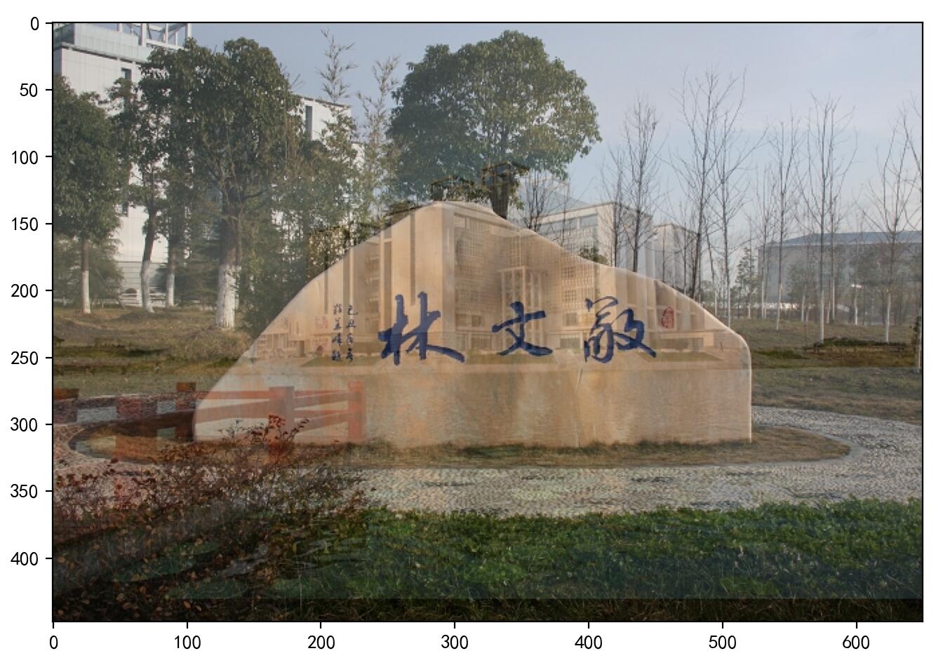
现在我们把两幅图混合在一起。第一幅图的权重是0.7,第二幅图的权重是0.3。函数
cv2.addWeighted()可以按下面的公式对图片进行混合操作。- 这里取为零。
  import numpy as np
  import cv2 as cv
  import matplotlib.pyplot as plt

  # 1 读取图像

   img1 = cv.imread("./images/002.jpg")
   img2 = cv.imread("./images/001.jpg")
   img2.resize(img1.shape)

  # 2 图像混合
  img3 = cv.addWeighted(img1,0.7,img2,0.3,0)

  # 3 图像显示
  plt.figure(figsize=(8,8))
  plt.imshow(img3[:,:,::-1])
  plt.show()
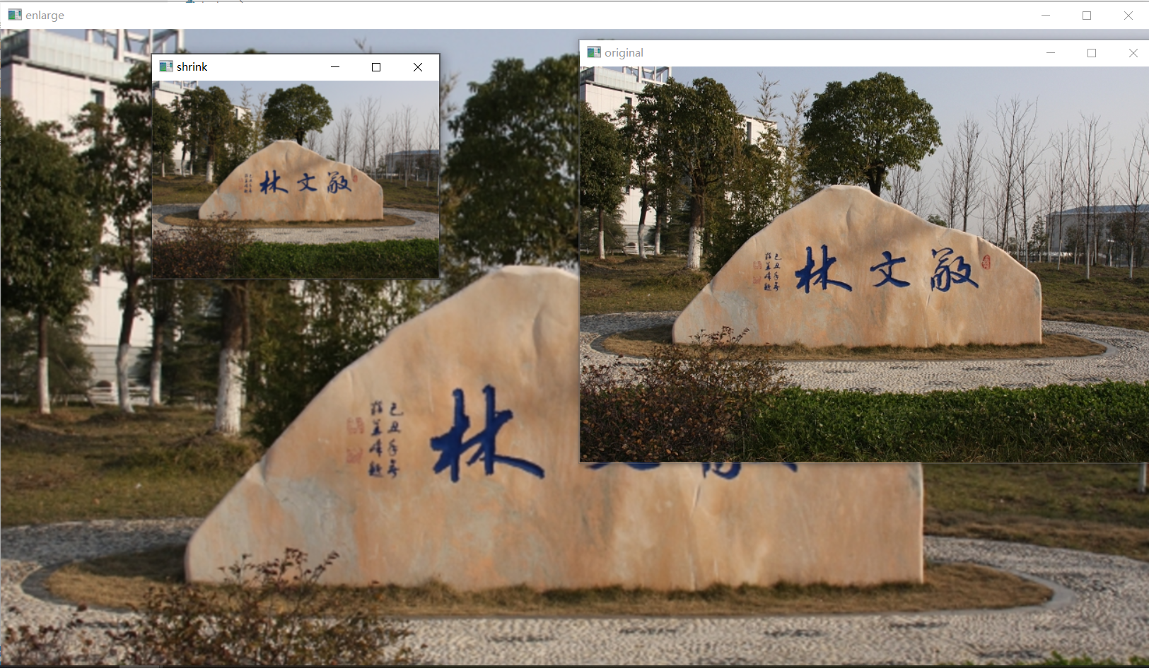
1.2.3. 图像缩放
缩放是对图像的大小进行调整,即使图像放大或缩小
cv2.resize(src,dsize,fx=0,fy=0,interpolation=cv2.INTER_LINEAR)参数:
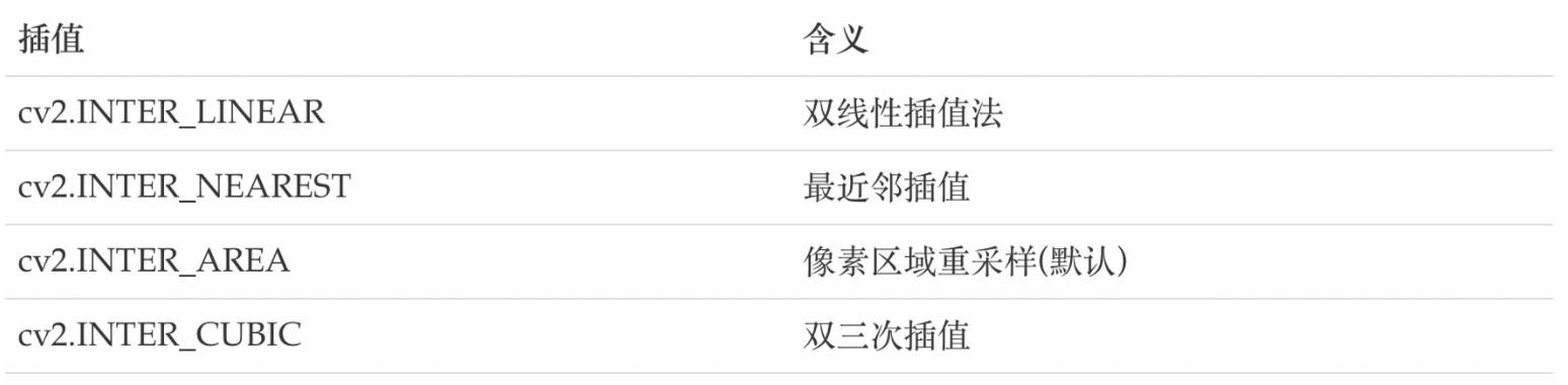
src: 输入图像dsize: 绝对尺寸,直接指定调整后图像的大小fx,fy:相对尺寸,将dsize设置为None,然后将fx和fy设置为比例因子即可interpolation:插值方法
import numpy as np
import cv2 as cv
import matplotlib.pyplot as plt

# 1. 读取图片
img1 = cv.imread("./images/001.jpg")
# 2.图像缩放
# 2.1 绝对尺寸
rows,cols = img1.shape[:2]
res = cv.resize(img1,(2*cols,2*rows),interpolation=cv.INTER_CUBIC)

# 2.2 相对尺寸
res1 = cv.resize(img1,None,fx=0.5,fy=0.5)

# 3 图像显示
# 3.1 使用opencv显示图像(不推荐)
cv.imshow("orignal",img1)
cv.imshow("enlarge",res)
cv.imshow("shrink",res1)
cv.waitKey(0)

# 3.2 使用matplotlib显示图像
fig,axes=plt.subplots(nrows=1,ncols=3,figsize=(10,8),dpi=100)
axes[0].imshow(res[:,:,::-1])
axes[0].set_title("绝对尺度(放大)")
axes[1].imshow(img1[:,:,::-1])
axes[1].set_title("原图")
axes[2].imshow(res1[:,:,::-1])
axes[2].set_title("相对尺度(缩小)")
plt.show()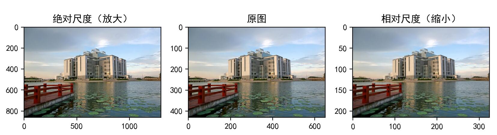
1.2.4. 图像平移
图像平移将图像按照指定方向和距离,移动到相应的位置
cv.warpAffine(img,M,dsize)
参数:
img: 输入图像
M: 2*3移动矩阵
对于(x,y)处的像素点,要把它移动到$(x+t_x , y+t_y)$处时,
M矩阵应如下设置: 注意:将M设置为np.float32类型的Numpy数组。dsize: 输出图像的大小注意:输出图像的大小,它应该是(宽度,高度)的形式。请记住,width=列数,height=行数。
将图像的像素点移动(50,100)的距离:
import numpy as np
import cv2 as cv
import matplotlib.pyplot as plt
import matplotlib
matplotlib.rcParams["font.sans-serif"]=["SimHei"]

# 1. 读取图像
img1 = cv.imread("./images/002.jpg")

# 2. 图像平移
rows,cols = img1.shape[:2]
M = M = np.float32([[1,0,100],[0,1,50]])# 平移矩阵
dst = cv.warpAffine(img1,M,(cols,rows))

# 3. 图像显示
fig,axes=plt.subplots(nrows=1,ncols=2,figsize=(10,8),dpi=100)
axes[0].imshow(img1[:,:,::-1])
axes[0].set_title("原图")
axes[1].imshow(dst[:,:,::-1])
axes[1].set_title("平移后结果")
plt.show()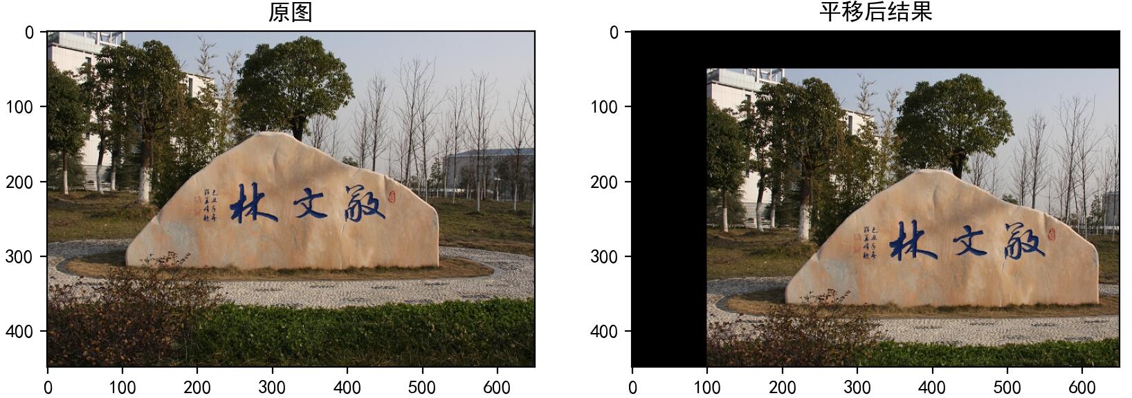
1.2.5. 图像旋转
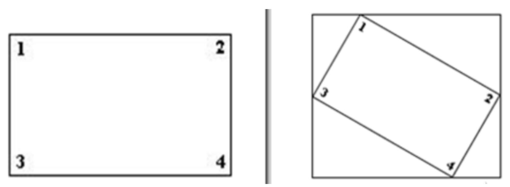
图像旋转是指图像按照某个位置转动一定角度的过程,旋转中图像仍保持这原始尺寸。
图像旋转后图像的水平对称轴、垂直对称轴及中心坐标原点都可能会发生变换,因此需要对图像旋转中的坐标进行相应转换
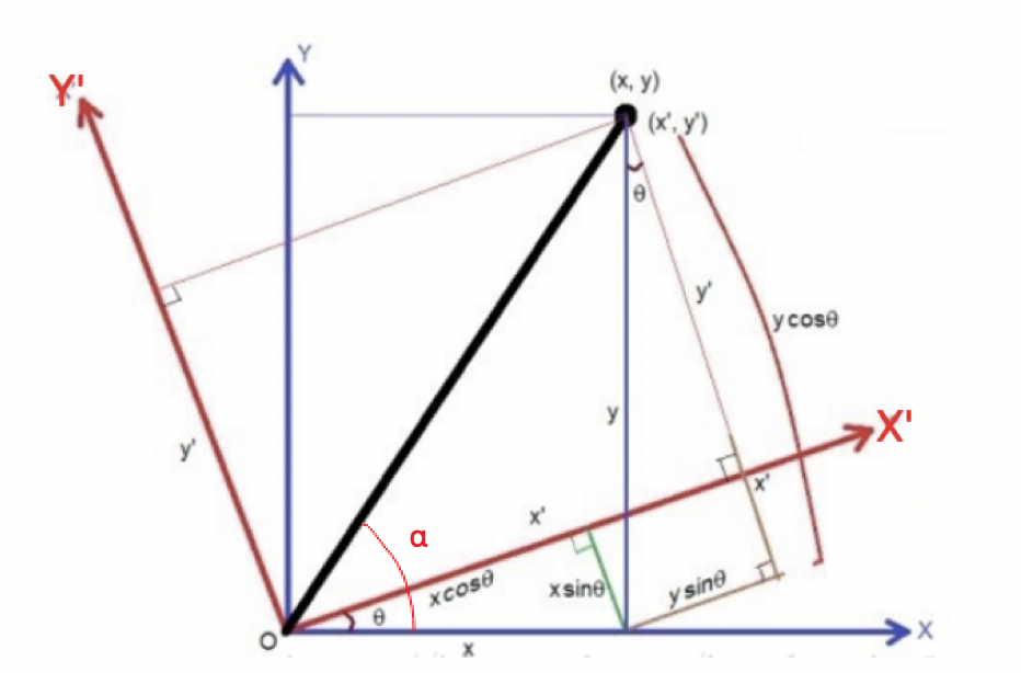
其中: 带入上面的公式中,则: 表示成矩阵的形式为:
假设在旋转的时候是以旋转中心为坐标原点的,旋转结束后还需要将坐标原点移到图像左上角,也就是还要进行一次变换
在OpenCV中图像旋转首先根据旋转角度和旋转中心获取旋转矩阵,然后根据旋转矩阵进行变换,即可实现任意角度和任意中心的旋转效果。
cv2.getRotationMatrix2D(center, angle, scale)参数:
- center:旋转中心
- angle:旋转角度
- scale:缩放比例
返回:
M:旋转矩阵
调用
cv.warpAffine完成图像的旋转
import numpy as np
import cv2 as cv
import matplotlib.pyplot as plt
# 1 读取图像
img = cv.imread("./image2/001.jpg")

# 2 图像旋转
rows,cols = img.shape[:2]
# 2.1 生成旋转矩阵
M = cv.getRotationMatrix2D((cols/2,rows/2),60,1)
# 2.2 进行旋转变换
dst = cv.warpAffine(img,M,(cols,rows))

# 3 图像展示
fig,axes=plt.subplots(nrows=1,ncols=2,figsize=(10,8),dpi=100)
axes[0].imshow(img[:,:,::-1])
axes[0].set_title("原图")
axes[1].imshow(dst[:,:,::-1])
axes[1].set_title("旋转后结果")
plt.show()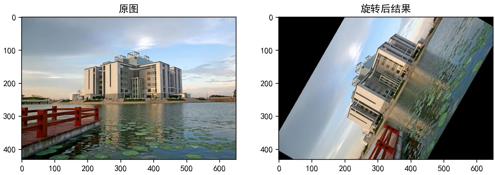
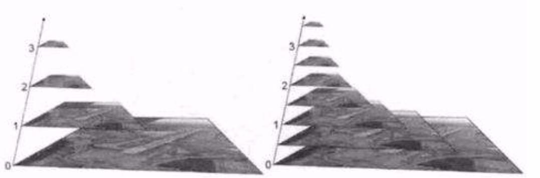
1.2.6. 图像金字塔
图像金字塔是图像多尺度表达的一种,最主要用于图像的分割,是一种以多分辨率来解释图像的有效但概念简单的结构。
图像金字塔用于机器视觉和图像压缩,一幅图像的金字塔是一系列以金字塔形状排列的分辨率逐步降低,且来源于同一张原始图的图像集合。其通过梯次向下采样获得,直到达到某个终止条件才停止采样。
金字塔的底部是待处理图像的高分辨率表示,而顶部是低分辨率的近似,层级越高,图像越小,分辨率越低。
cv.pyrUp(img)       #对图像进行上采样
cv.pyrDown(img)     #对图像进行下采样
import numpy as np
import cv2 as cv
import matplotlib.pyplot as plt
# 1 图像读取
img = cv.imread("./images/002.jpg")
# 2 进行图像采样
up_img = cv.pyrUp(img)  # 上采样操作
img_1 = cv.pyrDown(img)  # 下采样操作
# 3 图像显示
cv.imshow('enlarge', up_img)
cv.imshow('original', img)
cv.imshow('shrink', img_1)
cv.waitKey(0)
cv.destroyAllWindows()
1.3. 实验步骤
按照以上实验内容,对images文件夹的图像进行以下,并截图和记录实验结果:
- 读取图像
- 将任意两幅图像进行混合,混合比率为0.6,0.4,将最终的结果保存为图片,名称为
blend.jpg - 对
blend.jpg图像进行平移 (120,20),将最终结果保存为trans_blend.jpg - 对
trans_blend.jpg图像进行缩放0.8,将最终结果保存为sca_trans_blend.jpg - 对
scal_trans_blend.jpg图像进行旋转40度,将最终结果保存为rot_scal_trans_blend.jpg - 对
rot_scal_trans_blend.jpg图像分别进行上采样和下采样,将结果分别保存为up.jpg和down.jpg - 以上结果图片均需要嵌入自己的学号和姓名
- 提交实验报告,实验报告中的结果图片均需要嵌入学号和姓名
- 提交实验代码,代码应该适当进行注释
- 将结果(实验结果(6张图片)+实验报告+
code.py)打包上传到学习通平台上